How to perform normality test in r studio

What is normality test?

A normality test is used to determine whether sample data has been drawn from a normally distributed population (within some tolerance). A number of statistical tests, such as the Student's t-test and the one-way and two-way ANOVA require a normally distributed sample population. If the assumption of normality is not valid, the results of the tests will be unreliable.

There are some ways for testing normality:

A. Normal probability Q-Q plot.

A normal probability plot, or more specifically a quantile-quantile (Q-Q) plot, shows the distribution of the data against the expected normal distribution.

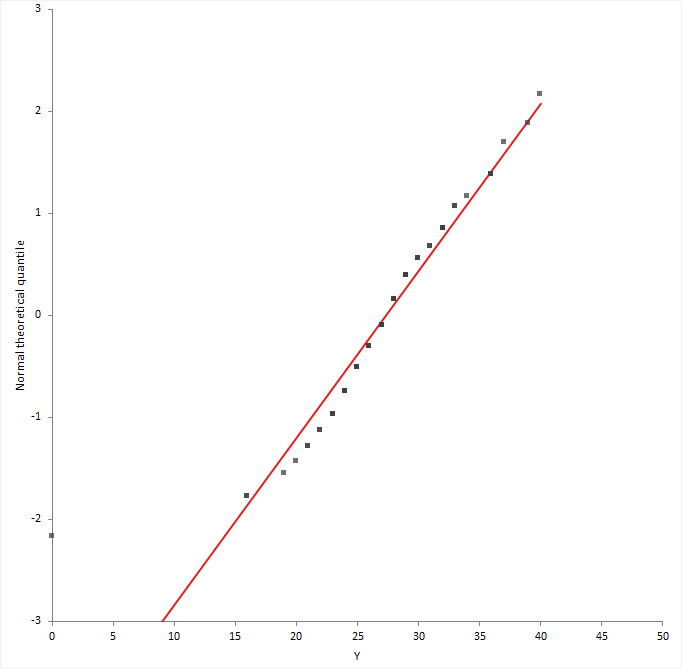
The above figure shows how it look like. 

It’s just a visual check, not an air-tight proof, so it is somewhat subjective. But it allows us to see at-a-glance if our assumption is plausible, and if not, how the assumption is violated and what data points contribute to the violation. Here is how the qq plot might look like.

Quantiles represent points in a dataset below which a certain portion of the data fall. For example, the 0.9 quantile represents the point below which 90% of the data fall below. The 0.5 quantile represents the point below which 50% of the data fall below, and so on.

If the data points fall along a straight diagonal line in a Q-Q plot, then the dataset likely follows a normal distribution.

B.Normality test

1. Shapiro-Wilk: Common normality test, but does not work well with duplicated data or large sample sizes.
2. Kolmogorov-Smirnov: For testing Gaussian distributions with specific mean and variance.
3. Lilliefors: Kolmogorov-Smirnov test with corrected P. Best for symmetrical distributions with small sample sizes.
4. Anderson-Darling: Can give better results for some datasets than Kolmogorov-Smirnov.
5. D'Agostino's K-Squared: Based on transformations of sample kurtosis and skewness. Especially effective for “non-normal” values.
6. Chen-Shapiro: Extends Shapiro-Wilk test without loss of power. Supports limited sample size (10 ≤ n ≤ 2000).

1. Kolmogorov-Smirnov: The K-S test, though known to be less powerful, is widely used. Generally, it requires large sample sizes.
2. Kolmogorov-Smirnov-Lilliefors: An adaptation of the K-S test. More complicated than K-S, since it must be established whether the maximum discrepancy between empirical distribution function and the cumulative distribution function is large enough to be statistically significant. K-S-L is generally recommended over K-S. Some analysts recommend that the sample size of K-S-L be larger than 2000.
3. Anderson-Darling: One of the best EDF-based statistics for normality testing. Sample size of less than 26 is recommended, but industrial data with 200 and more might pass A-D. The p-value of the A-D test depends on simulation algorithms. The A-D test can be used to test for other distributions with other specified simulation plans. See D’Agostino and Stephens (1986) for details.
4. D'Agostino K-Squared: Based on skewness and kurtosis measures. See D’Agostino, Belanger, and D’Agostino, Jr. (1990) and Royston (1991) for details. It is worthwhile mentioning that skewness and kurtosis are also affected by sample size.
5. Shapiro-Wilk: The recommended sample size for this test ranges from 7 to 2000. Origin allows sample sizes from 3 to 5000. However, when sample size is relatively large, D'Agostino K-squared or Lilliefors are generally preferred over Shapiro-Wilk.
6. Chen-Shapiro: The C-S test extends the S-W test without loss of power. The motivation for C-S is based on the fact that the ratios of the sample spacing to their expected spacing would converge to one due to the consistency of sample quantiles. From the standpoint of power, C-S performs more like the S-W test rather than the S-F test.

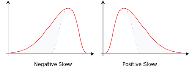
The Shapiro-Wilk test is a way to tell if a random sample comes from a normal distribution. The test gives you a W value; small values indicate your sample is not normally distributed (you can reject the null hypothesis that your population is normally distributed if your values are under a certain threshold). The formula for the W value is:

where:
xi are the ordered random sample values
ai are constants generated from the covariances, variances and means of the sample (size n) from a normally distributed sample.

It is recommended to use the test along with normal probability curve. This test is however effected by sample size.

Interpretation: If the P value of Shapiro test is more than 0.05, the data is normally distributed. If it is less than 0.05, there is deviation from normal distribution. 

C. Normality curve and histogram

Is the shape of the histogram normal? The following characteristics of normal distributions.

1. The first characteristic of the normal distribution is that the mean  (average), median , and mode  are equal.
2. A second characteristic of the normal distribution is that it is symmetrical. This means that if the distribution is cut in half, each side would be the mirror of the other. It also must form a bell-shaped curve  to be normal. A bimodal  or uniform  distribution may be symmetrical; however, these do not represent normal distributions.
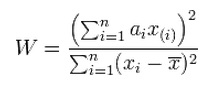
3. A third characteristic of the normal distribution is that the total area under the curve is equal to one. The total area, however, is not shown. This is because the tails extend to infinity. Standard practice is to show 99.73% of the area, which is plus and minus 3 standard deviations  from the average.



Figure: Standard deviation and normal curve



4. The fourth characteristic of the normal distribution is that the area under the curve can be determined. If the spread of the data (described by its standard deviation) is known, one can determine the percentage of data under sections of the curve. To illustrate, refer to the sketches right. For Figure A, 1 times the standard deviation to the right and 1 times the standard deviation to the left of the mean (the center of the curve) captures 68.26% of the area under the curve. For Figure B, 2 times the standard deviation on either side of the mean captures 95.44% of the area under the curve. Consequently, for Figure C, 3 times the standard deviation on either side of the mean captures 99.73% of the area under the curve. These percentages are true for all data that falls into a normally distributed pattern. These percentages are found in the standard normal distribution table.
5. Once the mean and the standard deviation of the data are known, the area under the curve can be described. For instance 3 times the standard deviation on either side of the mean captures 99.73% of the data.

Follow these steps to interpret histograms.

1. Study the shape.
2. Calculate descriptive statistics.
3. Compare the histogram to the normal distribution.

4. 

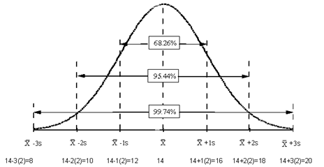
   Figure: Skewed distribution
   
   
   

   

   Figure: Normal distribution curve (bell shaped and tails are equal)
   
   
   

   
   

   Normality check in R Studio: 

1. First need to attach : 

import file

attach(filename) e.g. Practice

2. Observe histogram (I have written the variable as yield_before):  

hist(variable) e.g. hist(yield_before) 

hist(yield_before,breaks = 12,col = "green")

3. See QQ plot

qqnorm(yield_before);qqline(yield_before)

4. Normality check with Shapiro and other test: 

shapiro.test(yield_before)

#Output is given below: 

Shapiro-Wilk normality test

data:  yield_before

W = 0.88419, p-value = 0.05482

Note: As the P value is more than 0.05 we can assume normality. 

library(nortest)

ad.test(yield_before)  note: It is for Anderson Darling test 

#Output is shown below

Anderson-Darling normality test

data:  yield_before

A = 0.6554, p-value = 0.06971

5. Outliers detection: 

library(rstatix)

t%>%

  group_by(Treatment) %>% 

  identify_outliers(yield_before)

#Output is obtained as below: 

[1] Treatment    yield_before yield_after  is.outlier   is.extreme  

<0 rows> (or 0-length row.names)

# As we cannot see values in outliers and extreme outliers, there is nothing to worry about. 

6. Histogram and normal curve

g=yield_before

hist(g)

m<-mean(g)

hist(g)

m<-mean(g)

std<-sqrt(var(g))

hist(g, density=20, breaks=12, prob=TRUE, 

     xlab="x-variable", ylim=c(0, 0.0015), 

     main="normal curve over histogram")

Figure: Histogram with its density

curve(dnorm(x, mean=m, sd=std), 

      col="red", lwd=2, add=TRUE, yaxt="n")

Figure: Normal curve over histogram

# Interpretation: It is approximately normal distributed. 

7. Boxplot

boxplot(yield_before~Treatment,xlab = "Treatment",ylab = "yield of okra")

Figure: Box plot

or

 bxp<-ggboxplot(t,x="Treatment",y="yield_before",add = "point")

> bxp

#Note: t is the file name. 

Figure: Boxplot

We can also see it in color shades:

bxp<-ggboxplot(t,x="Treatment",y="yield_before",color = "Treatment",palette = "jco")

bxp

Figure: Colorful box plot

8. Way of seeing P value of normality by other way: 

library(psych)

library(pastecs)

describe(g)

#Output is seen as such:

   vars  n    mean     sd median trimmed    mad min  max range  skew kurtosis

X1    1 15 1390.67 592.84   1600 1413.08 667.17 390 2100  1710 -0.51     -1.2

       se

X1 153.07

stat.desc(g,basic = FALSE,norm = TRUE)

       median          mean       SE.mean  CI.mean.0.95           var       std.dev 

 1.600000e+03  1.390667e+03  1.530716e+02  3.283060e+02  3.514638e+05  5.928438e+02 

     coef.var      skewness      skew.2SE      kurtosis      kurt.2SE    normtest.W 

 4.263019e-01 -5.058726e-01 -4.360073e-01 -1.198214e+00 -5.344888e-01  8.841922e-01 

   normtest.p 

 5.481970e-02 

# Note: See the P value, for normal distribution, it should be more than 0.05.


Note : The tutorial video for testing the normality is given below.

https://www.youtube.com/watch?v=FXRiVtVw5Hs

The file for practice is given below:

https://drive.google.com/file/d/1DLZSRrkdDTkc4yEHHvEnzJ2zSt3-D1Do/view?usp=sharing