Experimental design analysis with R (CRD and RCBD)

1. Some definitions  before we start : 

Statistics is defined as the science of collecting, analyzing, and drawing conclusions from data. Data is usually collected through sampling surveys, observational studies, or experiments.

Experiment is the scientifically planned method to draw a valid conclusion about a particular problem. The variation due to environmental factor or uncontrolled factor is called as experimental error. 

Experimental Unit is the item under study upon which something is changed. This could be raw materials, human subjects, or just a point in time. It is the small plot of the block to which the treatment can be applied. 

Design: Whenever an experiment is done by using certain scientific (statistical ) procedure, it is called as design. It can also be defined as the various types of plot arrangements which are used to test a set of treatments to draw a valid conclusion about a particular problem. 

Treatment: The objects under comparison are called treatments. 

The choice of treatment, the method of assigning treatments to experimental units and the arrangement of experimental units in various pattern to suit the requirements of a particular problem is called as design of experiment. It is also the process of planning and study to meet the specific objectives. Experimental design was first introduced by prof. R.A. Fischer in 1920. 

Why experimental design?

• increase precision of experiment
• reduce experimental error
• in screening of various treatments
• in partitioning of variation into different components
• used in proper interpretation of scientific results and drawing  valid conclusion
• in reducing soil heterogeneity
•  in assessment of variance and covariance 
• shows the direction of better results
• includes the plan of analysis and reporting the results 

Can see more of the design in the following slide:
https://www.slideshare.net/DevendraKumar375/experimental-design-in-plant-breeding

2. What is experimental research? 

Experimental research is research conducted with a scientific approach using two sets of variables. The first set acts as a constant, which you use to measure the differences of the second set. Quantitative research methods, for example, are experimental.

Types of experimental research design

The classic experimental design definition is, “The methods used to collect data in experimental studies.”

There are three primary types of experimental design:

• Pre-experimental research design
• True experimental research design
• Quasi-experimental research design

The way you classify research subjects, based on conditions or groups, determines the type of design.

A. Pre-experimental research design: A group, or various groups, are kept under observation after implementing factors of cause and effect. You’ll conduct this research to understand whether further investigation is necessary for these particular groups.

You can break down pre-experimental research further in three types:

• One-shot Case Study Research Design
• One-group Pretest-posttest Research Design
• Static-group Comparison

B. True experimental research design: True experimental research relies on statistical analysis to prove or disprove a hypothesis, making it the most accurate form of research. Of the types of experimental design, only true design can establish a cause-effect relationship within a group. In a true experiment, three factors need to be satisfied:

• There is a Control Group, which won’t be subject to changes, and an Experimental Group, which will experience the changed variables.
• A variable which can be manipulated by the researcher
• Random distribution

Experimental design is applied in many areas, and methods have been tailored to the needs of various fields. This task view starts out with a section on the historically earliest application area, agricultural experimentation. Subsequently, it covers the most general packages, continues with specific sections on industrial experimentation, computer experiments, and experimentation in the clinical trials contexts (this section is going to be removed eventually; experimental design packages for clinical trials will be integrated into the clinical trials task view), and closes with a section on various special experimental design packages that have been developed for other specific purposes. 

C. Quasi-experimental research design: The word “Quasi” indicates similarity. A quasi-experimental design is similar to experimental, but it is not the same. The difference between the two is the assignment of a control group. In this research, an independent variable is manipulated, but the participants of a group are not randomly assigned. Quasi-research is used in field settings where random assignment is either irrelevant or not required.

3. Principle of experimentation 

Almost all experiments involve the three basic principles, viz., randomization, replication and local control. These three principles are, in a way, complementary to each other in trying to increase the accuracy of the experiment and to provide a valid test of significance, retaining at the same time the distinctive features of their roles in any experiment. Before we actually go into the details of these three principles, it would be useful to understand certain generic terms in the theory experimental designs and also understand the nature of variation among observations in an experiment.

These principles make a valid test of significance possible. Each of them is described briefly in the following subsections.

•  Randomization. The first principle of an experimental design is randomization, which is a random process of assigning treatments to the experimental units. The random process implies that every possible allotment of treatments has the same probability. An experimental unit is the smallest division of the experimental material, and a treatment means an experimental condition whose effect is to be measured and compared. The purpose of randomization is to remove bias and other sources of extraneous variation which are not controllable. Another advantage of randomization (accompanied by replication) is that it forms the basis of any valid statistical test. Hence, the treatments must be assigned at random to the experimental units. 
• Replication. The second principle of an experimental design is replication, which is a repetition of the basic experiment. In other words, it is a complete run for all the treatments to be tested in the experiment. In all experiments, some kind of variation is introduced because of the fact that the experimental units such as individuals or plots of land in agricultural experiments cannot be physically identical. This type of variation can be removed by using a number of experimental units. We therefore perform the experiment more than once, i.e., we repeat the basic experiment. An individual repetition is called a replicate. The number, the shape and the size of replicates depend upon the nature of the experimental material. A replication is used to:

       (i) Secure a more accurate estimate of the experimental error, a term which represents   the differences that would be observed if the same treatments were applied several times to the same experimental units;

       (ii)Decrease the experimental error and thereby increase precision, which is a measure of the variability of the experimental error; and

      (iii) Obtain a more precise estimate of the mean effect of a treatment.

• Local Control. It has been observed that all extraneous sources of variation are not removed by randomization and replication. This necessitates a refinement of the experimental technique. In other words, we need to choose a design in such a manner that all extraneous sources of variation are brought under control. For this purpose, we make use of local control, a term referring to the amount of balancing, blocking and grouping of the experimental units. Balancing means that the treatments should he assigned to the experimental units in such a way that the result is a balanced arrangement of the treatments. Blocking means that like experimental units should be collected together to form a relatively homogeneous group. We first divide field into several homogeneous parts known as blocks. A block is also a replicate. The main purpose of the principle of local control is to increase the efficiency of an experimental design by decreasing the experimental error. The point to remember here is that the term local control should not be confused with the word control. The word control in experimental design is used for a treatment which does not receive any treatment when we need to find out the effectiveness of other treatments through comparison.

What is completely randomized design? 

A completely randomized design (CRD) is one where the treatments are assigned completely at random so that each experimental unit has the same chance of receiving any one treatment. For the CRD, any difference among experimental units receiving the same treatment is considered as experimental error. Hence, CRD is appropriate only for experiments with homogeneous experimental units, such as laboratory experiments, where environmental effects are relatively easy to control. For field experiments, where there is generally large variation among experimental plots in such environmental factors as soil, the CRD is rarely used.

Analysis of variance for CRD

Figure: ANOVA for single factor CRD

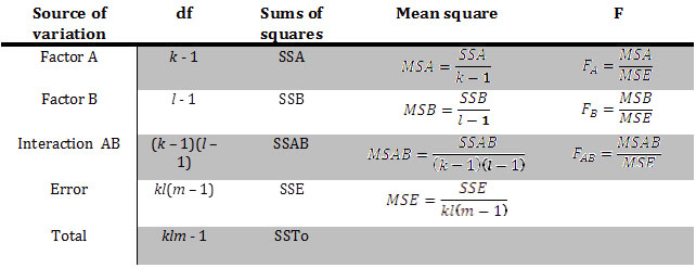Figure: ANOVA for 2 factors in CRD 

What is randomized completely block design?

The RCBD is the standard design for agricultural experiments where similar experimental units are grouped into blocks or replicates. It is used to control variation in an experiment by accounting for spatial effects in the  field .

The field or space is divided into uniform units to account for any variation so that observed differences are largely due to true differences between treatments. Treatments are then assigned at random to the subjects in the blocks-once in each block. The defining feature of the Randomized Complete Block Design is that each block sees each treatment exactly once. 

Advantages of the RCBD 

• Generally more precise than the completely randomized design (CRD). 
• No restriction on the number of treatments or replicates. 
• Some treatments may be replicated more times than others. 
• Missing plots are easily estimated. 

Disadvantages of the RCBD 

• Error degrees of freedom is smaller than that for the CRD (problem with a small number of treatments). 
• Large variation between experimental units within a block may result in a large error term.
• If there are missing data, a RCBD experiment may be less efficient than a CRD.

Things you should keep in mind about RCBD

• The number of blocks is the number of replications.
• Treatments are assigned at random within blocks of adjacent subjects, each treatment once per block.
• Any treatment can be adjacent to any other treatment, but not to the same treatment within the block .  

Layout of RCBD

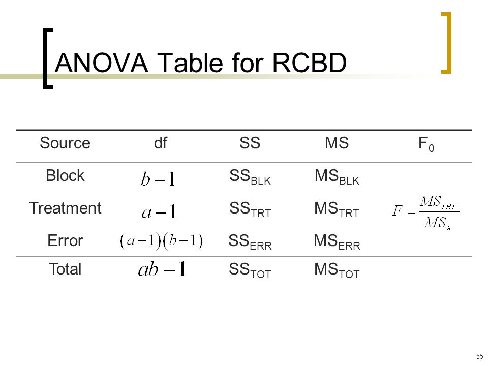
ANOVA for RCBD

Posthoc test

The original solution to this problem, developed by Fisher, was to explore all possible pair-wise comparisons of means comprising a factor using the equivalent of multiple t-tests. This procedure was named the Least Significant Difference (LSD) test.  LSD or minimum difference between a pair of means necessary for statistical significance.

For experiments, requiring the comparison of all possible pairs of treatment means, the LSD test is usually not suitable, when the total number of treatment is large. In such cases, DMRT is useful. DMRT involves the computation of numerical boundaries, that allow for the classification of the difference between any 2 treatment means as significant or non-significant. This requires calculation of a series of values each corresponding to a specific set of pair comparisons. Various steps, data and analysis for DMRT are as given by Gomez and Gomez (1984).

Calculation is shown in the given sites: 

https://www.statisticshowto.com/post-hoc/

https://www.statisticshowto.com/tukey-test-honest-significant-difference/

https://www.statisticshowto.com/how-to-calculate-the-least-significant-difference-lsd/

https://www.statisticshowto.com/duncans-multiple-range-test/ 

Analysis of CRD in R studio

Single factor : Use file crd.xls  (Output is in blue color). 
https://drive.google.com/file/d/1xCBBC3yczaiSL0Obpm4f-H2c_6qIBgqh/view?usp=sharing

> attach(crd1)

> head(crd1)

# A tibble: 6 x 2

  Treatment Yield

  <chr>     <dbl>

1 T1          4.5

2 T2          4.8

3 T3          5.2

4 T4          5.6

5 T5          6.2

6 T6          6.3

> crd1$Treatment <- as.factor(crd1$Treatment)

> crd1

# A tibble: 18 x 2

   Treatment Yield

   <fct>     <dbl>

 1 T1          4.5

 2 T2          4.8

 3 T3          5.2

 4 T4          5.6

 5 T5          6.2

 6 T6          6.3

 7 T1          4.9

 8 T2          4.7

 9 T3          5.4

10 T4          5.8

11 T5          6.5

12 T6          6.7

13 T1          4.3

14 T2          4.6

15 T3          4.9

16 T4          5.8

17 T5          6.4

18 T6          6.6

Now run ANOVA (please check for normality before it) 

> model<- aov(Yield~Treatment)  

> summary(model)

                       Df   Sum Sq    Mean Sq     F value        Pr(>F)    

Treatment    5      10.484      2.0969       51.01         1.14e-07 ***

Residuals      12     0.493      0.0411                     

---

Signif. codes:  0 ‘***’ 0.001 ‘**’ 0.01 ‘*’ 0.05 ‘.’ 0.1 ‘ ’ 1

#Interpretation: As our P value is less than 0.05 we can conclude that the yield was significantly different among treatments. So, we will be doing mean separation. 

Before that, See error (residual) degree of freedom and mean sum of square (from example df=12, Mse=0.0411) 

For mean separation you can select LSD or DMRT or Tukey HSD or any other ways.  You need to install agricolae package. 

> library(agricolae)

> out<-duncan.test(model,"Treatment")

> out

$statistics

     MSerror Df     Mean      CV

  0.04111111 12 5.511111 3.67909

$parameters

    test    name.t ntr alpha

  Duncan Treatment   6  0.05

$duncan

     Table CriticalRange

2 3.081307     0.3607064 (note this is the LSD value) 

3 3.225244     0.3775561

4 3.312453     0.3877651

5 3.370172     0.3945218

6 3.410202     0.3992079

$means

      Yield       std r Min Max  Q25 Q50  Q75

T1 4.566667 0.3055050 3 4.3 4.9 4.40 4.5 4.70

T2 4.700000 0.1000000 3 4.6 4.8 4.65 4.7 4.75

T3 5.166667 0.2516611 3 4.9 5.4 5.05 5.2 5.30

T4 5.733333 0.1154701 3 5.6 5.8 5.70 5.8 5.80

T5 6.366667 0.1527525 3 6.2 6.5 6.30 6.4 6.45

T6 6.533333 0.2081666 3 6.3 6.7 6.45 6.6 6.65

$comparison

NULL

$groups

      Yield groups

T6 6.533333      a

T5 6.366667      a

T4 5.733333      b

T3 5.166667      c

T2 4.700000      d

T1 4.566667      d

attr(,"class")

[1] "group"

Interpretation: The highest yield was obtained for treatment T6 which was at par with T5 but significantly higher than other treatments. The lowest yield was obtained for T1. The coefficient of variation was 3.67%. 

Analysis of RCBD in R studio

File used: rcbd1
Link: https://drive.google.com/file/d/1X6qz3S4HRfdu8iDTIHnMHMOZNjSbU7vs/view?usp=sharing

Import and attach as previous
> rcbd1$treatment<-as.factor(rcbd1$treatment)
> rcbd1
# A tibble: 20 x 3
   Block treatment Yield
   <chr> <fct>     <dbl>
 1 R1    T1          4.5
 2 R1    T2          4.8
 3 R1    T3          5.2
 4 R1    T4          5.6

 5 R1    T5          6.2
 6 R2    T1          4.7
 7 R2    T2          4.9
 8 R2    T3          5.2
 9 R2    T4          5.7
10 R2    T5          6  
11 R3    T1          4.5
12 R3    T2          4.8
13 R3    T3          5.3
14 R3    T4          5.7
15 R3    T5          6.1
16 R4    T1          4.6
17 R4    T2          4.9
18 R4    T3          5.2
19 R4    T4          5.7

20 R4    T5          6.1

> model<-aov(Yield~Block+treatment)
> summary(model)
                    Df          Sum Sq       Mean Sq      F value   Pr(>F)    
Block           3           0.005         0.0018          0.328    0.805    
treatment   4           6.053         1.5132          271.030 1.19e-11 ***
Residuals   12         0.067         0.0056                     
---

Signif. codes:  0 ‘***’ 0.001 ‘**’ 0.01 ‘*’ 0.05 ‘.’ 0.1 ‘ ’ 1

#Interpretation: There is significant difference among treatments. See error df and Mse.

> library(agricolae)
> out1<-with(rcbd1,LSD.test(Yield,treatment,DFerror = 12,MSerror =0.0056))
> out1
$statistics
  MSerror     Df      Mean       CV             t.value                LSD
   0.0056      12       5.285      1.415954   2.178813         0.1152919

$parameters
        test p.ajusted    name.t ntr alpha
  Fisher-LSD      none treatment   5  0.05

$means
   Yield        std r      LCL      UCL Min Max   Q25  Q50   Q75
T1 4.575 0.09574271 4 4.493476 4.656524 4.5 4.7 4.500 4.55 4.625
T2 4.850 0.05773503 4 4.768476 4.931524 4.8 4.9 4.800 4.85 4.900
T3 5.225 0.05000000 4 5.143476 5.306524 5.2 5.3 5.200 5.20 5.225
T4 5.675 0.05000000 4 5.593476 5.756524 5.6 5.7 5.675 5.70 5.700
T5 6.100 0.08164966 4 6.018476 6.181524 6.0 6.2 6.075 6.10 6.125

$comparison
NULL

$groups
   Yield groups
T5 6.100      a
T4 5.675      b
T3 5.225      c
T2 4.850      d
T1 4.575      e

Interpretation: The yield of T5 is significantly higher than other treatments. 

It can also be done by Duncan test. Which is given below
> out2<-with(rcbd1,duncan.test(Yield,treatment,DFerror = 12,MSerror =0.0056))
> out2
$statistics
  MSerror       Df        Mean       CV
   0.0056        12        5.285     1.415954

$parameters
    test    name.t ntr alpha
  Duncan treatment   5  0.05

$duncan
     Table CriticalRange
2 3.081307     0.1152919
3 3.225244     0.1206776
4 3.312453     0.1239406
5 3.370172     0.1261003

$means
   Yield        std r Min Max   Q25  Q50   Q75
T1 4.575 0.09574271 4 4.5 4.7 4.500 4.55 4.625
T2 4.850 0.05773503 4 4.8 4.9 4.800 4.85 4.900
T3 5.225 0.05000000 4 5.2 5.3 5.200 5.20 5.225
T4 5.675 0.05000000 4 5.6 5.7 5.675 5.70 5.700

T5 6.100 0.08164966 4 6.0 6.2 6.075 6.10 6.125

$comparison
NULL

$groups
   Yield groups
T5 6.100      a
T4 5.675      b
T3 5.225      c
T2 4.850      d

T1 4.575      e

For Tukey test, it can be done as below: 

> summary(fm1 <- aov(Yield ~ Block + treatment, data = rcbd1))

            Df Sum Sq Mean Sq F value   Pr(>F)    
Block        3  0.005  0.0018   0.328    0.805    
treatment    4  6.053  1.5132 271.030 1.19e-11 ***
Residuals   12  0.067  0.0056                     
---
Signif. codes:  0 ‘***’ 0.001 ‘**’ 0.01 ‘*’ 0.05 ‘.’ 0.1 ‘ ’ 1


> TukeyHSD(fm1, "treatment", ordered = TRUE)
  Tukey multiple comparisons of means
    95% family-wise confidence level
    factor levels have been ordered

Fit: aov(formula = Yield ~ Block + treatment, data = rcbd1)

$treatment
                   diff            lwr              upr              p adj
T2-T1     0.275      0.1065881 0.4434119        0.0016731
T3-T1    0.650      0.4815881 0.8184119       0.0000003
T4-T1   1.100      0.9315881 1.2684119      0.0000000
T5-T1   1.525      1.3565881 1.6934119      0.0000000
T3-T2    0.375    0.2065881 0.5434119     0.0001003
T4-T2   0.825    0.6565881 0.9934119    0.0000000
T5-T2   1.250    1.0815881 1.4184119     0.0000000
T4-T3   0.450    0.2815881 0.6184119     0.0000161
T5-T3   0.875   0.7065881 1.0434119     0.0000000

T5-T4   0.425    0.2565881 0.5934119     0.0000289

or
> model.tables(model, "means")
Tables of means
Grand mean
      
5.285 

 Block 
Block
  R1   R2   R3   R4 

5.26 5.30 5.28 5.30 

> TukeyHSD(model)
(you will get the same output)

>plot(TukeyHSD(fm1,"treatment"))

Analysis for 2 factor crd (file used: crd2f.xlsx)

https://drive.google.com/file/d/1-bkkP87zsKqrwBmdqHJaJwwMMRKK8joz/view?usp=sharing
> attach(crd2f)
> crd2f$factorA<-as.factor(crd2f$factorA)
>crd2f$FactorB<-as.factor(crd2f$FactorB)
> str(crd2f)
tibble [24 x 5] (S3: tbl_df/tbl/data.frame)
 $ factorA                      : Factor w/ 2 levels "S1","S2": 1 1 1 1 1 1 1 1 1 1 ...
 $ FactorB                      : Factor w/ 3 levels "P0","P1","P2": 1 1 1 1 2 2 2 2 3 3 ...
 $ Plant height                 : num [1:24] 133 133 140 135 128 ...
 $ No.of branches               : num [1:24] 17 16 15 18 17 19 22 18 18 20 ...
 $ Days to flower bud initiation: num [1:24] 68 65 67 63 75 78 80 70 95 98 ...
> model1<-aov(`Plant height`~factorA+FactorB+factorA:FactorB)
> summary(model1)
                Df Sum Sq Mean Sq F value   Pr(>F)    
factorA          1  127.6   127.6   3.678      0.071140 .  

FactorB          2  801.0   400.5  11.547 0.000593 ***
factorA:FactorB  2  246.4   123.2   3.552 0.050109 .  
Residuals       18  624.3    34.7                     
---

Signif. codes:  0 ‘***’ 0.001 ‘**’ 0.01 ‘*’ 0.05 ‘.’ 0.1 ‘ ’ 1

Interpretation: See the significance for factor B. See error df . Though there was not significance for factor A,  I am running it for your convenience. 

> library(agricolae)
> out<-with(crd2f,duncan.test(`Plant height`,factorA,DFerror = 18,MSerror = 34.7))
> out
$statistics
  MSerror      Df          Mean     CV
     34.7         18 129.     1389   4.5615

$parameters
    test  name.t ntr alpha
  Duncan factorA   2  0.05

$duncan
     Table CriticalRange
2 2.971152      5.052415

$means
   Plant height       std  r      Min      Max      Q25      Q50    Q75
S1     131.4444  5.127352 12 123.3333 139.6667 127.9167 132.3333 135.00

S2     126.8333 11.211014 12 104.6667 143.6667 121.2500 123.8333 134.75

$comparison
NULL

$groups
   Plant height groups
S1     131.4444      a
S2     126.8333      a

attr(,"class")

[1] "group"

Interpretation: There is no significance difference for factor A.

Again, we will run command for factor B:

> out1<-with(crd2f,duncan.test(`Plant height`,FactorB,DFerror = 18,MSerror = 34.7))
> out1
$statistics
  MSerror Df     Mean     CV
     34.7 18 129.1389 4.5615

$parameters
    test  name.t ntr alpha
  Duncan FactorB   3  0.05

$duncan
     Table CriticalRange
2 2.971152      6.187920
3 3.117384      6.492472

$means
   Plant height      std r      Min      Max      Q25      Q50      Q75
P0     136.9167 4.527703 8 131.0000 143.6667 133.0000 137.0000 140.0000
P1     127.4167 5.980797 8 120.0000 136.6667 123.1666 125.8333 132.0833
P2     123.0833 9.291999 8 104.6667 135.0000 120.5834 123.8333 127.9167

$comparison
NULL

$groups
   Plant height groups
P0     136.9167      a
P1     127.4167      b

P2     123.0833      b

Interpretation: The height of Po is significantly higher than other two factors P1 and P2.  

(Note: Similar letters signify that there is no significant difference among P1 and P2). 

Now lets do it for interaction: (though there is no significance observed)

> out1<-with(crd2f,duncan.test(`Plant height`,factorA:FactorB,DFerror = 18,MSerror = 34.7))
> out1
$statistics
  MSerror Df     Mean     CV
     34.7 18 129.1389 4.5615

$parameters
    test          name.t ntr alpha
  Duncan factorA:FactorB   6  0.05

$duncan
     Table CriticalRange
2 2.971152      8.751040
3 3.117384      9.181742
4 3.209655      9.453510
5 3.273593      9.641828
6 3.320327      9.779476

$means
      Plant height      std r      Min      Max      Q25      Q50      Q75
S1:P0     135.1667 3.144676 4 133.0000 139.6667 133.0000 134.0000 136.1667
S1:P1     130.0000 5.610869 4 123.3333 136.6667 127.0833 130.0000 132.9167
S1:P2     129.1667 5.181890 4 123.3333 135.0000 125.8334 129.1667 132.5000
S2:P0     138.6667 5.456912 4 131.0000 143.6667 137.0000 140.0000 141.6667
S2:P1     124.8333 5.846792 4 120.0000 133.3333 122.0000 123.0000 125.8333
S2:P2     117.0000 8.713529 4 104.6667 124.3333 114.1666 119.5000 122.3334

$comparison
NULL

$groups
      Plant height groups
S2:P0     138.6667      a
S1:P0     135.1667     ab
S1:P1     130.0000    abc
S1:P2     129.1667     bc
S2:P1     124.8333     cd

S2:P2     117.0000      d

Lets do it for RCBD also: 

File name:Rcbd2

https://drive.google.com/file/d/1WT4uCS378d-Hp_Gtu19C24V1fEHDZxRR/view?usp=sharing

Don't forget to import, attach and read it as factor as shown above.

> model3<-aov(`Plant height`~Rep+factorA+FactorB+factorA:FactorB)
>summary(model3)
                                            Df        Sum Sq          Mean Sq         F value          Pr(>F)   
Rep                                      3         6.2                     2.1              0.050         0.98442   
factorA                                1       127.6               127.6               3.096        0.09886 . 

FactorB                               2       801.0             400.5               9.720        0.00196 **
factorA:FactorB                2       246.4              123.2               2.989       0.08078 . 
Residuals                          15       618.1                41.2                   
---

Signif. codes:  0 ‘***’ 0.001 ‘**’ 0.01 ‘*’ 0.05 ‘.’ 0.1 ‘ ’ 1

> out2<-with(rcbd2,duncan.test(`Plant height`,FactorB,DFerror = 15,MSerror = 41.2))
> out2
$statistics
  MSerror          Df               Mean              CV
     41.2 15         12                9.1389        4 .970402

$parameters
    test  name.t ntr alpha
  Duncan FactorB   3  0.05

$duncan
     Table CriticalRange
2 3.014325      6.840592

3 3.159826      7.170787

$means
   Plant height      std r      Min      Max      Q25      Q50      Q75
P0     136.9167 4.527703 8 131.0000 143.6667 133.0000 137.0000 140.0000
P1     127.4167 5.980797 8 120.0000 136.6667 123.1666 125.8333 132.0833
P2     123.0833 9.291999 8 104.6667 135.0000 120.5834 123.8333 127.9167

$comparison
NULL

$groups
   Plant height groups
P0     136.9167      a
P1     127.4167      b

P2     123.0833      b

Interpretation: Height of Po is significantly higher than other two. 

I hope you can do similarly for others; factor A and interaction

More over, the link of videos below will also help you in this regard.

https://www.youtube.com/watch?v=oL5zLnh6qb0&t=6611s

https://www.youtube.com/watch?v=MVYRLpmxH48&t=2491s