Split plot and strip plot analysis in R studio

What is Split Plot design? 

A split plot design is a special case of a factorial treatment structure. It is used when some factors are harder (or more expensive) to vary than others. In simple terms, a split-plot experiment is a blocked experiment, where the blocks themselves serve as experimental units for a subset of the factors.Thus, there are two levels of experimental units. The blocks are referred to as whole plots, while the experimental units within blocks are called split plots, split units, or subplots. Corresponding to the two levels of experimental units are two levels of randomization. One randomization is conducted to determine the assignment of block-level treatments to whole plots. Then, as always in a blocked experiment, a randomization of treatments to split-plot experimental units occurs within each block or whole plot. 

Split plot design has a mixture of hard to randomize ( hard to change) and easy to randomize (easy to change) factors. The hard to change factors are implemented first and followed by easy to change factors. It was invented by Fischer in 1975. This type of design is seen in agriculture, industries and medical fields. It is appropriate for all those studies where you find it difficult to change or randomize a factor. Split plot design is generally used when factors are not of same importance. 

Example. An experiment is to compare the yield of three varieties of Moong bean (factor A with a=3 levels) and four different levels of manure (factor B with b=4 levels). Suppose 6 farmers agree to participate in the experiment and each will designate a farm field for the experiment (blocking factor with s=6 levels). Since it is easier to plant a variety of moong bean in a large field, the experimenter uses a split-plot design as follows:

•  To divide each block into three equal sized plots (whole plots), and each plot is assigned a variety of oat according to a randomized block design. 
• Each whole plot is divided into 4 plots (split-plots) and the four levels of manure are randomly assigned to the 4 splitplots. 
• We  call varieties level the whole-plot factor and manure level as  the split-plot factor.
• Whole plots are the experimental units for whole plot factor and split plots for split plot factor.

If we are seeing the effect of irrigation (whole) and variety of maize (split) on yield, the model will be as below:

Note: Observation in the same whole plot shares whole plot error. Precision is more in this type. 

For every “level” (whole-plot / split-plot) of the experiment we have to introduce a corresponding random effect (better terminology: error) which acts as the experimental error on that level.  To identify the correct design we have to know the randomization procedure. The general situation can be very complex, but by following the different randomization levels/steps, setting up a model is easy. 

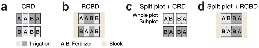
a) In CRD, levels of irrigation and fertilizer are assigned to plots of land (experimental units) in a random and balanced fashion. (b) In RCBD, similar experimental units are grouped (for example, by field) into blocks and treatments are distributed in a CRD fashion within the block. (c) If irrigation is more difficult to vary on a small scale and fields are large enough to be split, a split plot design becomes appropriate. Irrigation levels are assigned to whole plots by CRD and fertilizer is assigned to subplots using RCBD (irrigation is the block). (d) If the fields are large enough, they can be used as blocks for two levels of irrigation. Each field is composed of two whole plots, each composed of two subplots. Irrigation is assigned to whole plots using RCBD (blocked by field) and fertilizer assigned to subplots using RCBD (blocked by irrigation).

Source: https://www.nature.com/articles/nmeth.3293/figures/1

 Split plot designs are usually used with factorial sets when the assignment of treatments at random can cause difficulties

–        large scale machinery required for one factor but not another

•          irrigation

•          tillage

–        plots that receive the same treatment must be grouped together

•          for a treatment such as planting date, it may be necessary to group treatments to facilitate field operations

The split plot is a design which allows the levels of one factor to be applied to large plots while the levels of another factor are applied to small plots

–        Large plots are whole plots or main plots

–        Smaller plots are split plots or subplots

 Levels of the whole-plot factor are randomly assigned to the main plots, using a different randomization for each block (for an RBD).  Levels of the subplots are randomly assigned within each main plot using a separate randomization for each main plot.

ü  Because there are two sizes of plots, there are two experimental errors - one for each size plot

ü  Usually the sub plot error is smaller and has more df

ü  Therefore the main plot factor is estimated with less precision than the subplot and interaction effects

ü  Precision is an important consideration in deciding which factor to assign to the main plot

Advantages

ü  Permits the efficient use of some factors that require different sizes of plot for their application

ü  Permits the introduction of new treatments into an experiment that is already in progress

Disadvantages

ü  Main plot factor is estimated with less precision so larger differences are required for significance – may be difficult to obtain adequate df for the main plot error

ü  Statistical analysis is more complex because different standard errors are required for different comparisons

Design of Split plots:

There are two blocks, 3 main plot factors (varieties) and 4 subplot factors (varieties) in the figure above. 

ANOVA for split plots

F ratios in Split plot design

ü  F ratios are computed somewhat differently because there are two errors

ü  F_R=MSR/MSE_A   tests the effectiveness of blocking

ü  F_A=MSA/MSE_A  tests the sig. of the A main effect

ü  F_B=MSB/MSE_B   tests the sig. of the B main effect

ü  F_AB=MSAB/MSE_B tests the sig. of the AB interaction

Variations of split plot design

ü  Split-plot arrangement of treatments could be used in a CRD or Latin Square, as well as in an RBD

ü  Could extend the same principles to accommodate another factor in a split-split plot (3-way factorial)

ü  Could add another factor without an additional split (3-way factorial, split-plot arrangement of treatments)

What is Strip plot design?

 Strip plots are also called as split-block design. For experiments involving factors that are difficult to apply to small plots. There are three sizes of plots so there are three experimental errors. The interaction is measured with greater precision than the main effects.  For example:

Ø  Three seed-bed preparation methods

Ø  Four nitrogen levels

Ø  Both factors will be applied with large scale machinery

  Advantages

  ü  Permits efficient application of factors that would be difficult to apply to small plots

Disadvantages 

ü  Differential precision in the estimation of interaction and the main effects

 ü Complicated statistical analysis

ANOVA for strip plot

In strip plot design, the desired precision for measuring the interaction effect between the two factors is higher than that for measuring the main effect of either one of the two factors. This is accomplished with the use of three plot sizes:

ü  Vertical strip plot for the first factor also called the vertical factor.

ü  Horizontal strip plot for the second factor also called the horizontal factor.

ü  Intersection plot for the interaction between the two factors.

The vertical strip and horizontal strip plot are always perpendicular to each other. However, there is no relationship between their sizes, unlike the case of main plot and subplot of the split-plot design. In this case, the interaction plot is, of course, the smallest.

In strip plot design, the degrees of precision associated with the main effects of both factors are sacrificed in order to improve the precision of the interaction effect.  But, in the split-plot design, the levels of the second factor or factor B are independently randomized within the subplots of each level of the first factor or factor A. In the strip plot design the levels of one factor are assigned to strip plots in one direction and the levels of the second factor to the strips perpendicular to the first strip. A separate randomization is done for each block for each factor A and B. This design facilitates the physical operations and increases the precision for estimation of the interaction effect.

Split plot vs strip plot

3 varieties and 4 fertilizer dose are considered for experiment. The varieties are taken as main plots whereas fertilizers as subplots. Then the layout for one block indicates the difference between split plot and strip plot as shown below:

R Commands for Split plots

File used: split.xls https://drive.google.com/file/d/1eGIeKlXWHpnPqeTiihsVcGIQAznM6jZu/view?usp=sharing
Note: The output are shown in blue color. 

1. Import  and attach data set 
> split <- read_excel("D:/google/data analysis/r/split.xls")
> attach(split)

2. Observe your data
> head(split)
# A tibble: 6 x 7
  Rep   Fa            Fb             Ph1   pdi   ch1   ch2
  <chr> <chr>  <chr>        <dbl> <dbl> <dbl> <dbl>
1 R1    Ganesh Jholmal       6.1  0.777  51.5  31.5
2 R1    Ganesh Azadirachtin  5.38 0.999  40.6  36.4
3 R1    Ganesh Imidacloprid  6.28 0.624  43.0  39.0
4 R1    Ganesh Cow's milk    3.55 0.777  46.2  38.1
5 R1    Ganesh Control       3.68 0.777  45.9  35.1
6 R1    Bramha Jholmal       3.9  0.555  46.2  40.7

Note: The factor A and B are set as characters 

3. Set Characters as factors

> split$Fa <- as.factor(split$Fa)
> split$Fb <- as.factor(split$Fb)
> str(split)
tibble [75 x 7] (S3: tbl_df/tbl/data.frame)
 $ Rep: chr [1:75] "R1" "R1" "R1" "R1" ...
 $ Fa : Factor w/ 5 levels "Bishnu","Bramha",..: 3 3 3 3 3 2 2 2 2 2 ...
 $ Fb : Factor w/ 5 levels "Azadirachtin",..: 5 1 4 3 2 5 1 2 4 3 ...
 $ Ph1: num [1:75] 6.1 5.38 6.28 3.55 3.67 ...
 $ pdi: num [1:75] 0.777 0.999 0.624 0.777 0.777 ...
 $ ch1: num [1:75] 51.5 40.6 43 46.2 45.9 ...
 $ ch2: num [1:75] 31.5 36.4 39 38.1 35.1 ...

Note: Factor A and B have been converted into factors. 

4. Now run command for ANOVA 

> library(agricolae)
> aov<-with(split,sp.plot(Rep,Fa,Fb,ch2)) 

ANALYSIS SPLIT PLOT:  ch2 
Class level information

Fa :  Ganesh Bramha Riddi Bishnu Laxmi 
Fb :  Jholmal Azadirachtin Imidacloprid Cow's milk Control 
Rep :  R1 R2 R3 

Number of observations:  75 

Analysis of Variance Table

Response: ch2
           Df         Sum Sq       Mean Sq         F value      Pr(>F)    
Rep     2          163.45            81.73         1.8723    0.2152758    
Fa       4         1816.36         454.09        10.4031    0.0029443 ** 
Ea       8          349.20           43.65                          
Fb       4          737.16  1       84.29         6.1032     0.0006241 ***
Fa:Fb 16         561.12           35.07       1.1614       0.3379647    
Eb      40       1207.83          30.20                      
---
Signif. codes:  0 ‘***’ 0.001 ‘**’ 0.01 ‘*’ 0.05 ‘.’ 0.1 ‘ ’ 1

cv(a) = 16 %, cv(b) = 13.3 %, Mean = 41.40167 

Interpretation: The chlorophyll content is significantly different (P<0.001) for both factors i.e. main factor and split factor. 

Note: Though the significant difference was not seen for interaction effect, I will be showing the analysis and output for you. 

5. Now perform mean separation

a. For Main effect (variety) 

> out<-with(split,duncan.test(ch2,Fa,DFerror = 8,MSerror = 43.65))

> out

$statistics

  MSerror        Df        Mean           CV

    43.65            8       41.40167     15.95785

Interpretation: The grand mean for factor A is 41.40 with CV of 15.95% 

$parameters

    test name.t ntr alpha

  Duncan     Fa   5  0.05

$duncan

     Table CriticalRange

2 3.261182      5.563160

3 3.398460      5.797338

4 3.475191      5.928231

5 3.521194      6.006707

Interpretation: The  LSD value is 5.563

$means

            ch2      std  r   Min   Max     Q25   Q50    Q75

Bishnu 44.84667 6.017778 15 35.21 53.61 40.0600 45.21 50.310

Bramha 43.63000 7.290326 15 25.61 53.81 40.7100 43.11 48.910

Ganesh 36.33000 5.838910 15 27.71 48.91 31.5475 36.41 38.535

Laxmi  47.36000 5.680229 15 38.66 56.01 43.4100 46.81 51.835

Riddi  34.84167 7.739812 15 22.61 54.31 30.1100 34.21 38.860

$comparison

NULL

$groups

            ch2 groups

Laxmi  47.36000       a

Bishnu 44.84667       a

Bramha 43.63000      a

Ganesh 36.33000       b

Riddi  34.84167         b

attr(,"class")

[1] "group"

Interpretation: The maximum chlorophyll content was seen for Laxmi variety which is significantly higher than Ganesh and Riddi but is at par with Bishnu and Bramha. 

b. For Split plot (pesticide) 

> out1<-with(split,duncan.test(ch2,Fb,DFerror = 40,MSerror = 30.20))

> out1

$statistics

  MSerror      Df        Mean         CV

    30.2           40       41.40167   13.27351

$parameters

    test name.t ntr alpha

  Duncan     Fb   5  0.05

$duncan

     Table CriticalRange

2 2.858232      4.055602

3 3.005302      4.264283

4 3.101506      4.400788

5 3.170852      4.499184

$means

                  ch2      std  r   Min   Max     Q25   Q50   Q75

Azadirachtin 40.54000 8.020833 15 22.61 53.81 36.7725 42.31 46.06

Control      40.03833 7.064365 15 29.61 52.36 34.6600 38.66 44.71

Cow's milk   39.86333 8.798746 15 24.91 52.11 34.4850 40.01 45.11

Imidacloprid 47.59000 7.623760 15 30.61 56.01 41.9100 51.51 52.91

Jholmal      38.97667 6.552281 15 25.61 51.11 35.0100 40.61 42.76

$comparison

NULL

$groups

                  ch2 groups

Imidacloprid 47.59000      a

Azadirachtin 40.54000      b

Control      40.03833         b

Cow's milk   39.86333      b

Jholmal      38.97667        b

attr(,"class")

Interpretation: The chlorophyll content is significantly higher in Imidacloprid sprayed plot than all other treatments. 

c. For interaction

> out2<-with(split,duncan.test(ch2,Fa*Fb,DFerror = 40,MSerror = 30.20))

> out2 

Note: I have not shown it here as significance was not observed in this case. 

OR

You need to first assign gla as model and gl.a is combined with dollar operator to represent error degree of freedom (8) for main plot factor. Similarly, assign glb to represent error degree of freedom (40) for the subplot factor and interaction term.

> gla<-aov$gl.a

> glb<-aov$gl.b

> Ea<-aov$Ea

> Eb<-aov$Eb

Now,  run the command as shown below:

> out1<-with(split,duncan.test(ch2,Fa,gla,Ea,console=TRUE))

> out2<-with(split,duncan.test(ch2,Fb,glb,Eb,console=TRUE))

> out3<-with(split,duncan.test(ch2,Fa:Fb,glb,Eb,console=TRUE))


We can also see error and bar graphs as shown below; 
> hist(ch2)
> bar.err(out1$means,variation="SE",ylim=c(0,60))

> bar.err(out2$means,variation="SE",ylim=c(0,60))

> bar.err(out3$means,variation="SE",ylim=c(0,60))

R commands for strip plots

File used: split.xls https://drive.google.com/file/d/1eGIeKlXWHpnPqeTiihsVcGIQAznM6jZu/view?usp=sharing

Note: Perform the first three commands as given for split plot.

1. Run ANOVA for strip plots

> aov<-with(split,strip.plot(Rep,Fa,Fb,ch2))

ANALYSIS STRIP PLOT:  ch2 

Class level information

Fa :  Ganesh Bramha Riddi Bishnu Laxmi 

Fb :  Jholmal Azadirachtin Imidacloprid Cow's milk Control 

Rep :  R1 R2 R3 

Number of observations:  75 

model Y: ch2 ~ Rep + Fa + Ea + Fb + Eb + Fb:Fa + Ec 

Analysis of Variance Table

Response: ch2

      Df  Sum Sq Mean Sq F value   Pr(>F)   

Rep    2  163.45   81.73  2.4980 0.098158 . 

Fa     4 1816.36  454.09 10.4031 0.002944 **

Ea     8  349.20   43.65  1.3342 0.262717   

Fb     4  737.16  184.29  9.1637 0.004412 **

Eb     8  160.89   20.11  0.6147 0.758865   

Fb:Fa 16  561.12   35.07  1.0719 0.417744   

Ec    32 1046.94   32.72                    

---

Signif. codes:  0 ‘***’ 0.001 ‘**’ 0.01 ‘*’ 0.05 ‘.’ 0.1 ‘ ’ 1

cv(a) = 16 %, cv(b) = 10.8 %, cv(c) = 13.8 %, Mean = 41.40167 

The mean separation is done by DMRT (duncan.test). Other options can also be used.  For main treatment factors, I have used error mean square and error degree of freedom respective to factor A and B from analysis of variance table. Similarly, for interaction error C for degree of freedom and its respective error mean square is used to compute.

For this objective, I assigned  gla as model and gl.a is combined with dollar operator to represent error degree of freedom (8) for the first factor. Similarly, assigned glb to represent error degree of freedom (8) for the second factor. Then assigned   glc to represent third error degree of freedom (32) for the interaction term. 

> gla<-model$gl.a

> glb<-model$gl.b

> glc<-model$gl.c

Moreover, for error mean square Ea was assigned as model and was combined with dollar operator. This gave the value of error mean square (23.734) for first factor. Similarly, Eb was assigned for representing error mean square (17.806) for second factor. Ec was assigned to represent error mean square (18.763) for interaction.

> Ea<-model$Ea

> Eb<-model$Eb

> Ec<-model$Ec

2. Now the mean separation can be done as follows: 

> out1<-with(split,duncan.test(ch2,Fa,gla,Ea))
> out1

If you don't want to do the steps mentioned above, you can do the following steps: 

> out1<-with(split,duncan.test(ch2,Fa,aov$gl.a,aov$Ea))

> out1

$statistics

   MSerror      Df          Mean                  CV

  43.64948        8      41.40167           15.95775

$parameters

    test name.t ntr alpha

  Duncan     Fa   5  0.05

$duncan

     Table       Critical  Range

2 3.261182      5.563127

3 3.398460      5.797304

4 3.475191      5.928196

5 3.521194      6.006671

$means

            ch2      std  r   Min   Max     Q25   Q50    Q75

Bishnu 44.84667 6.017778 15 35.21 53.61 40.0600 45.21 50.310

Bramha 43.63000 7.290326 15 25.61 53.81 40.7100 43.11 48.910

Ganesh 36.33000 5.838910 15 27.71 48.91 31.5475 36.41 38.535

Laxmi  47.36000 5.680229 15 38.66 56.01 43.4100 46.81 51.835

Riddi  34.84167 7.739812 15 22.61 54.31 30.1100 34.21 38.860

$comparison

NULL

$groups

                   ch2 groups

Laxmi         47.36000               a

Bishnu        44.84667               a

Bramha      43.63000               a

Ganesh       36.33000               b

Riddi          34.84167               b

attr(,"class")

[1] "group"

Interpretation: See grand mean, CV, LSD value and which variety is significantly different? ( I have made those values bold). 

> out6<-with(split,duncan.test(ch2,Fb,aov$gl.b,aov$Eb))

> out6

$statistics

   MSerror Df     Mean      CV

  20.11077  8 41.40167 10.8317

$parameters

    test name.t ntr alpha

  Duncan     Fb   5  0.05

$duncan

     Table CriticalRange

2 3.261182      3.776103

3 3.398460      3.935056

4 3.475191      4.023902

5 3.521194      4.077169

$means

                  ch2      std  r   Min   Max     Q25   Q50   Q75

Azadirachtin 40.54000 8.020833 15 22.61 53.81 36.7725 42.31 46.06

Control      40.03833 7.064365 15 29.61 52.36 34.6600 38.66 44.71

Cow's milk   39.86333 8.798746 15 24.91 52.11 34.4850 40.01 45.11

Imidacloprid 47.59000 7.623760 15 30.61 56.01 41.9100 51.51 52.91

Jholmal      38.97667 6.552281 15 25.61 51.11 35.0100 40.61 42.76

$comparison

NULL

$groups

                  ch2 groups

Imidacloprid 47.59000      a

Azadirachtin 40.54000      b

Control      40.03833      b

Cow's milk   39.86333      b

Jholmal      38.97667      b

attr(,"class")

[1] "group"

> 

> out7<-with(split,duncan.test(ch2,Fa:Fb,aov$gl.c,aov$Ec))

> out7

$statistics

   MSerror Df     Mean       CV

  32.71685 32 41.40167 13.81554

$parameters

    test name.t ntr alpha

  Duncan  Fa:Fb  25  0.05

$duncan

      Table CriticalRange

2  2.880659      9.512988

3  3.027689      9.998535

4  3.123222     10.314019

5  3.191582     10.539771

6  3.243335     10.710677

7  3.283984     10.844914

8  3.316744     10.953101

9  3.343648     11.041949

10 3.366058     11.115952

11 3.384925     11.178259

12 3.400942     11.231153

13 3.414625     11.276340

14 3.426369     11.315123

15 3.436482     11.348519

16 3.445208     11.377337

17 3.452745     11.402225

18 3.459253     11.423716

19 3.464864     11.442247

20 3.469690     11.458183

21 3.473823     11.471831

22 3.477342     11.483453

23 3.480344     11.493367

24 3.482802     11.501485

25 3.484829     11.508179

$means

                         ch2       std r    Min    Max     Q25    Q50     Q75

Bishnu:Azadirachtin 44.01833  6.134958 3 37.135 48.910 41.5725 46.010 47.4600

Bishnu:Control      42.51833  4.729715 3 38.510 47.735 39.9100 41.310 44.5225

Bishnu:Cow's milk   49.01000  5.026927 3 43.210 52.110 47.4600 51.710 51.9100

Bishnu:Imidacloprid 50.24333  4.441096 3 45.210 53.610 48.5600 51.910 52.7600

Bishnu:Jholmal      38.44333  2.853653 3 35.210 40.610 37.3600 39.510 40.0600

Bramha:Azadirachtin 46.44333  6.395571 3 42.310 53.810 42.7600 43.210 48.5100

Bramha:Control      41.71000  5.436911 3 35.710 46.310 39.4100 43.110 44.7100

Bramha:Cow's milk   45.97667  6.051722 3 40.010 52.110 42.9100 45.810 48.9600

Bramha:Imidacloprid 48.07667  6.384617 3 40.710 52.010 46.1100 51.510 51.7600

Bramha:Jholmal      35.94333  8.957864 3 25.610 41.510 33.1600 40.710 41.1100

Ganesh:Azadirachtin 34.68500  4.469550 3 29.610 38.035 33.0100 36.410 37.2225

Ganesh:Control      33.39333  1.834621 3 31.460 35.110 32.5350 33.610 34.3600

Ganesh:Cow's milk   32.45167  5.229145 3 27.710 38.060 29.6475 31.585 34.8225

Ganesh:Imidacloprid 43.67667  4.974267 3 39.010 48.910 41.0600 43.110 46.0100

Ganesh:Jholmal      37.44333  6.390879 3 31.510 44.210 34.0600 36.610 40.4100

Laxmi:Azadirachtin  45.67667  2.676440 3 42.810 48.110 44.4600 46.110 47.1100

Laxmi:Control       47.49333  7.663115 3 38.660 52.360 45.0600 51.460 51.9100

Laxmi:Cow's milk    41.57667  2.478575 3 39.810 44.410 40.1600 40.510 42.4600

Laxmi:Imidacloprid  54.74333  2.193931 3 52.210 56.010 54.1100 56.010 56.0100

Laxmi:Jholmal       47.31000  3.576311 3 44.010 51.110 45.4100 46.810 48.9600

Riddi:Azadirachtin  31.87667  8.405554 3 22.610 39.010 28.3100 34.010 36.5100

Riddi:Control       35.07667  5.947549 3 29.610 41.410 31.9100 34.210 37.8100

Riddi:Cow's milk    30.30167  6.407239 3 24.910 37.385 26.7600 28.610 32.9975

Riddi:Imidacloprid  41.21000 12.046161 3 30.610 54.310 34.6600 38.710 46.5100

Riddi:Jholmal       35.74333  4.572016 3 31.710 40.710 33.2600 34.810 37.7600

$comparison

NULL

$groups

                         ch2    groups

Laxmi:Imidacloprid  54.74333         a

Bishnu:Imidacloprid 50.24333        ab

Bishnu:Cow's milk   49.01000       abc

Bramha:Imidacloprid 48.07667      abcd

Laxmi:Control       47.49333      abcd

Laxmi:Jholmal       47.31000      abcd

Bramha:Azadirachtin 46.44333     abcde

Bramha:Cow's milk   45.97667    abcdef

Laxmi:Azadirachtin  45.67667    abcdef

Bishnu:Azadirachtin 44.01833   abcdefg

Ganesh:Imidacloprid 43.67667  abcdefgh

Bishnu:Control      42.51833  bcdefghi

Bramha:Control      41.71000  bcdefghi

Laxmi:Cow's milk    41.57667  bcdefghi

Riddi:Imidacloprid  41.21000 bcdefghij

Bishnu:Jholmal      38.44333  cdefghij

Ganesh:Jholmal      37.44333   defghij

Bramha:Jholmal      35.94333    efghij

Riddi:Jholmal       35.74333    efghij

Riddi:Control       35.07667     fghij

Ganesh:Azadirachtin 34.68500     fghij

Ganesh:Control      33.39333      ghij

Ganesh:Cow's milk   32.45167       hij

Riddi:Azadirachtin  31.87667        ij

Riddi:Cow's milk    30.30167         j

attr(,"class")

[1] "group"

Interpretation: Try to do it yourself. Same letter signify that they are not significantly different.