Analysis and interpretation of linear regression in R studio

 Linear regression is a statistical method used to model the relationship between a dependent variable and one or more independent variables by fitting a linear equation to the observed data. The goal of linear regression is to find the best-fit line that minimizes the sum of the squared differences between the observed values and the values predicted by the model.

The general form of a simple linear regression equation with one independent variable is:

$�={�}_0+{�}_1�+�$

where:

• $�$ is the dependent variable,
• $�$ is the independent variable,
• ${�}_0$ is the y-intercept,
• ${�}_1$ is the slope of the line,
• $�$ represents the error term.

Linear regression relies on several assumptions to ensure the validity of its results. Violations of these assumptions might affect the accuracy and reliability of the regression analysis. Here are the key assumptions of linear regression:

1. Linearity:

   • Assumption: The relationship between the independent variables and the dependent variable is linear.
   • Implication: The estimated regression coefficients represent the average change in the dependent variable for a one-unit change in the independent variable, assuming all other variables are held constant.

2. Independence of Residuals:

   • Assumption: Residuals (the differences between observed and predicted values) should be independent of each other.
   • Implication: The occurrence of one residual should not provide information about the occurrence of another. Independence ensures that the model is not missing important variables.

3. Homoscedasticity:

   • Assumption: Residuals should have constant variance across all levels of the independent variables.
   • Implication: The spread of residuals should be consistent, indicating that the variability of the dependent variable is constant across different levels of the independent variables.

4. Normality of Residuals:

   • Assumption: Residuals are normally distributed.
   • Implication: Normality is necessary for valid hypothesis testing and confidence intervals. Departures from normality may be less critical for large sample sizes due to the Central Limit Theorem.

5. No Perfect Multicollinearity:

   • Assumption: The independent variables should not be perfectly correlated with each other.
   • Implication: Perfect multicollinearity makes it challenging to estimate individual regression coefficients accurately.

6. No Autocorrelation:

   • Assumption: Residuals should not be correlated with each other (no serial correlation).
   • Implication: The occurrence of a residual at one point in time should not predict the occurrence of a residual at another point in time (for time-series data).

7. Additivity:

   • Assumption: The effect of changes in an independent variable on the dependent variable is consistent across all levels of other independent variables.
   • Implication: Each independent variable should have a consistent effect on the dependent variable, regardless of the values of other variables.

8. No Outliers or Influential Points:

   • Assumption: No extreme values (outliers or influential points) in the data.
   • Implication: Extreme values can disproportionately influence the regression results, affecting the accuracy of coefficient estimates.

Checking Assumptions:

• Diagnostic Plots: Residual plots, Q-Q plots, and others can help visually assess assumptions.

• Statistical Tests: Tests like the Shapiro-Wilk test for normality, Breusch-Pagan test for heteroscedasticity, and Durbin-Watson test for autocorrelation can be used to formally assess assumptions.

If assumptions are violated, corrective actions such as data transformations, inclusion of interaction terms, or using robust regression techniques might be considered. Additionally, understanding the context of the data and the potential implications of assumption violations is crucial in interpreting regression results.

In R, you can perform linear regression using the lm() function. Here's a simple example:

# Sample data set.seed(123) x <- rnorm(100) y <- 2*x + rnorm(100) # Fit linear regression model model <- lm(y ~ x) # Summary of the model summary(model)

Example:

# Set seed for reproducibility

set.seed(123)

# Create a simple dataset

ata <- data.frame(

  Y = rnorm(100, mean = 10, sd = 2),   # Dependent variable

  X1 = rnorm(100, mean = 5, sd = 2),   # Independent variable 1

  X2 = rnorm(100, mean = 8, sd = 3)    # Independent variable 2

)

# Perform linear regression

model <- lm(Y ~ X1 + X2, data = ata)

# Print summary of the model

summary(model)

This will create a dataset with 100 observations and perform a linear regression with the dependent variable Y and two independent variables X1 and X2.

Call:
lm(formula = Y ~ X1 + X2, data = ata)

Residuals:
    Min      1Q  Median      3Q     Max 
-4.5775 -1.2295 -0.1682  1.1247  4.6838 

Coefficients:
            Estimate Std. Error t value Pr(>|t|)    
(Intercept) 11.07138    0.71799  15.420   <2e-16 ***
X1          -0.04307    0.09499  -0.453    0.651    
X2          -0.08186    0.06447  -1.270    0.207    
---
Signif. codes:  0 ‘***’ 0.001 ‘**’ 0.01 ‘*’ 0.05 ‘.’ 0.1 ‘ ’ 1

Residual standard error: 1.827 on 97 degrees of freedom
Multiple R-squared:  0.01877,	Adjusted R-squared:  -0.001466 
F-statistic: 0.9276 on 2 and 97 DF,  p-value: 0.399

Now, let's perform some assumption tests:

# Install and load necessary packages install.packages("lmtest") library(lmtest) # Residuals vs Fitted Plot plot(model, which = 1)

# Normal Q-Q Plot plot(model, which = 2)

# Scale-Location Plot plot(model, which = 3)

# Residuals vs Leverage Plot plot(model, which = 5)

# Run Shapiro-Wilk test for normality of residuals shapiro.test(model$residuals)

Shapiro-Wilk normality test

data:  model$residuals
W = 0.99319, p-value = 0.899

# Run Breusch-Pagan test for heteroscedasticity bptest(model)

studentized Breusch-Pagan test

data:  model
BP = 2.744, df = 2, p-value = 0.2536

This code will generate the diagnostic plots and perform the Shapiro-Wilk test for normality of residuals and the Breusch-Pagan test for heteroscedasticity.

#Run Dublin Watson test

 durbinWatsonTest <- dwtest(model)
print(durbinWatsonTest)

Interpretation:

• The test statistic ranges from 0 to 4.
• A test statistic close to 2 indicates no autocorrelation.
• Values significantly below 2 suggest positive autocorrelation, while values significantly above 2 suggest negative autocorrelation.

For the Durbin-Watson test results, you typically focus on the test statistic and its significance level:

• If the test statistic is close to 2 and the p-value is high, there is no evidence of significant autocorrelation.
• If the test statistic is far from 2 and the p-value is low, it suggests the presence of autocorrelation.

Durbin-Watson test

data:  model
DW = 2.0343, p-value = 0.5699
alternative hypothesis: true autocorrelation is greater than 0

Since the test statistic is close to 2, and the p-value is relatively high, we do not have strong evidence to reject the null hypothesis of no autocorrelation.

So, now let's proceed further with an example.

We have used biodiversity.xlsx file.

1. Load and Explore the Data:

In the used file we have variables like production system, use of products and biodiversity percentage.

#Import the data and attach the file.

attach(biodiversity)

2. Fit a Multiple Linear Regression Model:

Use the lm() function to fit a multiple linear regression model:

# Fit the model model <- lm(`Bioversity percent`~ `Production system` + `Intended production`, data = biodiversity)

3. Interpret the Coefficients:

# Display summary of the model

summary(model)

The summary output will provide information about the coefficients, their standard errors, t-values, and p-values. Here's how you can interpret the key components:

• Coefficients: These represent the estimated effect of each variable on income.
• Standard Errors: Measure the precision of the coefficients.
• t-values: Indicate how many standard errors the coefficient is away from zero.
• P-values: Test the null hypothesis that the corresponding coefficient is zero.

Call:
lm(formula = `Bioversity percent` ~ `Production system` + `Intended production`, 
    data = biodiversity)

Residuals:
    Min      1Q  Median      3Q     Max 
-27.909  -8.584  -1.126   7.080  38.784 

Coefficients:
                                             Estimate Std. Error t value
(Intercept)                                    51.126      3.546  14.416
`Production system`Indigenous                  -4.193      3.040  -1.379
`Production system`Marginalized                -3.054      3.185  -0.959
`Intended production`Mostly sale               -0.849      4.732  -0.179
`Intended production`Mostly self-consumption   -4.467      4.233  -1.055
`Intended production`Self-consumption only    -14.456      3.967  -3.644
                                             Pr(>|t|)    
(Intercept)                                   < 2e-16 ***
`Production system`Indigenous                0.170567    
`Production system`Marginalized              0.339680    
`Intended production`Mostly sale             0.857947    
`Intended production`Mostly self-consumption 0.293528    
`Intended production`Self-consumption only   0.000408 ***
---
Signif. codes:  0 ‘***’ 0.001 ‘**’ 0.01 ‘*’ 0.05 ‘.’ 0.1 ‘ ’ 1

Residual standard error: 12.67 on 112 degrees of freedom
Multiple R-squared:  0.1961,	Adjusted R-squared:  0.1602 
F-statistic: 5.465 on 5 and 112 DF,  p-value: 0.0001542

• 1. Coefficients:

  • Intercept (51.126): The estimated mean value of the dependent variable (Bioversity percent) when all other predictors are zero.

  • Production system Indicators:

    • Indigenous (-4.193): The change in the mean Bioversity percent when the production system is Indigenous, compared to the reference category.
    • Marginalized (-3.054): The change in the mean Bioversity percent when the production system is Marginalized, compared to the reference category.

  • Intended production Indicators:

    • Mostly sale (-0.849): The change in the mean Bioversity percent when the intended production is Mostly sale, compared to the reference category.
    • Mostly self-consumption (-4.467): The change in the mean Bioversity percent when the intended production is Mostly self-consumption, compared to the reference category.
    • Self-consumption only (-14.456): The change in the mean Bioversity percent when the intended production is Self-consumption only, compared to the reference category.

  2. Pr(>|t|) (p-values):

  • Interpretation: Indicates the statistical significance of each coefficient. The smaller the p-value, the more evidence you have against a null hypothesis of no effect. In this case:
    • The Intercept is highly significant.
    • The indicator for Intended production as Self-consumption only is statistically significant (p-value = 0.000408), suggesting it has a significant impact on Bioversity percent.

  3. Residuals:

  • Min, 1Q, Median, 3Q, Max: Descriptive statistics of the residuals, showing the spread and central tendency.

  4. Residual Standard Error (12.67):

  • Interpretation: This is an estimate of the standard deviation of the residuals. It represents the average amount that actual values deviate from the predicted values.

  5. Multiple R-squared (0.1961) and Adjusted R-squared (0.1602):

  • Interpretation: Indicates the proportion of variance in the dependent variable (Bioversity percent) explained by the model. Adjusted R-squared considers the number of predictors in the model. In this case, the model explains approximately 16% of the variance.

  6. F-statistic (5.465) and p-value (0.0001542):

• Interpretation: Tests the overall significance of the model. The small p-value suggests that at least one predictor variable in the model has a significant effect on the dependent variable.

• 7. Shapiro-Wilk Test:

• Interpretation: The Shapiro-Wilk test tests the normality of residuals. A low p-value (< 0.05) suggests a departure from normality. If the p-value is not provided, run shapiro.test(model$residuals) separately.
• For above example:

• Shapiro-Wilk normality test
  
  data:  model$residuals
  W = 0.98035, p-value = 0.08166

• So, we assume that the residuals are normally distributed. 

Now, let's interpret the diagnostic plots for the given linear regression model:

# Assuming 'model' is the name of your linear regression model plot(model,1)

plot (model,2)

plot (model,3)

plot (model,4)

1. Residuals vs Fitted Plot:

• Interpretation: Check for a random scatter of points around the horizontal line at zero. The residuals should not show a clear pattern. It appears that there might be a slight U-shaped pattern in the residuals, suggesting a potential non-linear relationship that the current model might not capture well.
• 
  
  
  

2. Normal Q-Q Plot:

• Interpretation: Points on the Normal Q-Q plot should follow a straight line. In this case, the points deviate from a straight line in the tails, indicating a departure from normality. This suggests that the residuals are not perfectly normally distributed, especially in the tails.
• 
  
  
  

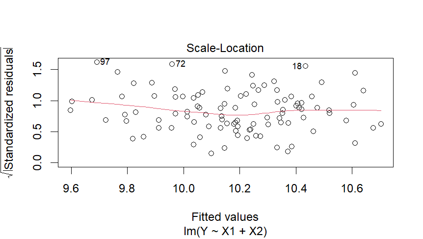
3. Scale-Location Plot:

• Interpretation: The spread of residuals should be consistent across different levels of fitted values. In your case, the spread looks somewhat consistent, indicating homoscedasticity. However, there might be a slight funnel shape, suggesting a possible issue with variance across fitted values.
• 
  
  
  

4. Residuals vs Leverage Plot:

• Interpretation: Check for influential points with high leverage and high residuals. In your plot, there doesn't seem to be any points with extremely high leverage or residuals. However, it's essential to investigate points that are close to the upper right corner, as they may have a larger impact on the model.
•