(Simple and multiple) linear regression & binary logistic regression in r studio
1. What is regression?
Regression is a measure of estimating the relationship between the mean value of one variable (output) and corresponding value of other variables. It is statistical method used in various disciplines in order to determine the strength and character of relationship between one dependent variable and a series of independent variables.2. Uses of regression
- It estimates the relationship between dependent variable and explanatory variable.
- Determine the effect of each explanatory variable on dependent variable by controlling the effect of other explanatory variables.
- Predict the value of dependent variable for a given value of explanatory variable.
- It is also used to forecast an effect and trend of future values.
3. What is linear regression?
In linear regression, the relationship between two variables is modeled by fitting a linear equation to the observed data. One variable is called as explanatory variable and the other one is dependent variable. Linear regression is basic and commonly used type of predictive analysis. The overall idea is to examine:
- how is independent variable predicting the outcome of dependent variable
- which independent variable is significantly affecting the outcome of dependent variable
- how does the magnitude and sign of beta estimates impact the dependent variable
Note: Dependent variables are often called as outcome variable, criterion variable, endogenous variable and regressand. Moreover, independent variables are also termed as exogenous variable, predictor variable and regressor.
The researcher should determine whether there is relationship between the variables of interest before attempting to fit the linear model to the observed data. It does not necessarily imply that one variable causes the other but there can be significant association between the variables. A scatter diagram is very useful in determining the strength of relationship between these variables. The increasing or decreasing trend is seen only if there is association between the proposed explanatory and dependent variables. The numerical measure of association between these variable is called as correlation coefficient whose value is between -1 and 1 . It shows the strength of association of the observed data.
 |
| Figure: Scatter diagram showing the type of relationship |
 |
Figure showing regression line and slope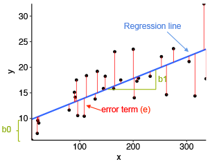 |
- blue line is best fit regression line
- the intercept (b0) and slope (b1) is shown in green
- the error term is represented by vertical red line
As shown in the figure above, some of the values are above blue line and some are below it which indicates that not all data points are fitted on regression line. The sum of squares of residuals is called as residual sum of squares. The average variation of points around the fitted regression line is called as residual standard error. It is important metric used to evaluate the quality of fitted regression model. Small value of this standard error is desirable.
4. Types of linear regression
- Simple linear regression: 1 dependent variable ( interval or ratio scale), 1 independent variable (interval or ratio or dichotomous)
The equation of linear equation is in the form of: Y=a+bX
Predicted Y’ =β0+β1X+ε …..>Simple Regression
Predicted Y’ =β0+β1X1+…+βnXn +ε …..>Multiple Regression
Where,
Y’ =Predicted value of dependent variable
β0 =Intercept
β1 =Regression coefficient (beta coefficient)
X =Independent (or explanatory) variable
ε =Error term
- Multiple linear regression: 1 dependent variable ( interval or ratio scale), 2+ independent variables (interval or ratio or dichotomous)
- Logistic regression: 1 dependent variable ( dichotomous), 2+ independent variables (interval or ratio or dichotomous)
The equation for logistic:
Logit(Y) = ln [Pi/(1- Pi)] = β0 + β1X1 +…+ βnXn
Logit(Y) = ln [Odds)] = β0 + β1X1 +…+ βnXn
where,
Logit(Y) =Predicted value of dependent variable
ln = Natural log
Pi =Probability of experiencing an event
(1-Pi) =Probability of not experiencing an event
Pi/(1-Pi) =Odds of experiencing an event
β0 =Intercept
β1 =Regression coefficient (Logit coefficient)
Xn =Independent (or explanatory) variable
Value of Odds Ratio Ranges from 0 to +∞
More than 1=Increased or higher odds
Less than 1=Decreased or lower odds
Equal to 1 = Same odds (no difference)
Value of Logit Coefficient ranges from -∞ to +∞
- =decreased logged odds
+ =increased logged odds
 |
| Figure showing logistic regression S curve for dichotomous dependent variable |
- Ordinal regression: 1 dependent variable ( ordinal), 1+ independent variable (s) (nominal or dichotomous)
- Multinomial regression: 1 dependent variable ( nominal), 1+ independent variable (s) (interval or ratio or dichotomous)
- Discrimiant analysis: 1 dependent variable ( nominal ), 1+ independent variable (interval or ratio)
5. Simple and multiple linear regression in R studio
A. For simple linear regression
File used: data.xlsx https://drive.google.com/file/d/1US3FfzF4LnKwf-fn-Om3pC80467N0iBu/view?usp=sharingNote: Output are shown in blue color
- Import the file in r studio
- Attach the file
> attach(data)
- Load required packages
> library(tidyverse)
> library(ggpubr)
> theme_set(theme_pubr())
> head(data,4)
# A tibble: 4 x 3
Nitrogen Mulching Yield
<dbl> <chr> <dbl>
1 0 No 15.7
2 20 No 18.2
3 30 No 20.5
4 40 No 24.5
- Now create a scatter plot displaying the Nitrogen dose versus yield of a crop and add a smoothed line.
> ggplot(data, aes(x = Nitrogen, y = Yield)) +
+ geom_point() +
+ stat_smooth()

There is almost linear relationship between Nitrogen and yield. One important assumption of linear regression that the relationship between dependent and independent variable is linear and additive is fulfilled.
We can also compute the correlation coefficient between the variables by using following function:
> cor(data$Yield, data$Nitrogen)
[1] 0.8748427
What we should know is that the correlation coefficient is calculated to measure the association between two variables whose value ranges from -1 to +1. -1 represents perfect negative correlation whereas +1 shows perfect positive correlation. Positive correlation is when X increases, Y also increases but in negative correlation increase on x will decrease the value in y. When the value of coefficient approaches 0, we can say that the relationship is weak. Generally coefficient between -2 and +2 is said to be weak. It suggests us that variation in dependent variable is not explained by independent variables and in such case we should look for other predictors.
In our case, there is strong relation as correlation coefficient is large enough suggesting us to build linear model "y as function of x".
- Computation of regression
In simple linear regression, we find the best line to predict yield with respect to dose of nitrogen. In this case the linear regression can be written as:
Yield=c+m*Nitrogen
In R studio, the function lm() is used to determine the coefficient of linear model
> model <- lm(Yield ~ Nitrogen, data = data)
> model
Call:
lm(formula = Yield ~ Nitrogen, data = data)
Coefficients:
(Intercept) Nitrogen
17.0643 0.2316
The result above shows the beta coefficient of Nitrogen (variable).
Interpretation;
The output states that the estimated regression line equation can be written as:
Yield=17.06+0.23*Nitrogen
Where
Intercept=17.06 which states that the predicted yield with 0 dose of nitrogen is 17.06 units.
Regression beta efficient=0.23 which is also known as slope. It means that each unit increase in dose of nitrogen increases the yield by 0.23 units.
- Regression line
> ggplot(data, aes(Nitrogen, Yield)) +
+ geom_point() +
+ stat_smooth(method = lm)
The above code can be used to add the regression line onto the scatter plot.

- Model assesment and its summary
We built the linear model of yield as function of nitrogen dose as ,
Yield=17.06+0.23*Nitrogen
But we can use this formula only if we are sure that our model is statistically significant. In other words, there is statistically significant relation between predictor and outcome variable and the model fits well the data. So, for it, we should check our regression model. It is done by following command.
> summary(model)
Call:
lm(formula = Yield ~ Nitrogen, data = data)
Residuals:
Min 1Q Median 3Q Max
-3.5114 -2.0350 -0.0271 2.2493 3.4571
Coefficients:
Estimate Std. Error t value Pr(>|t|)
(Intercept) 17.06429 1.57040 10.866 7.39e-07 ***
Nitrogen 0.23157 0.04055 5.711 0.000195 ***
---
Signif. codes: 0 ‘***’ 0.001 ‘**’ 0.01 ‘*’ 0.05 ‘.’ 0.1 ‘ ’ 1
Residual standard error: 2.77 on 10 degrees of freedom
Multiple R-squared: 0.7653, Adjusted R-squared: 0.7419
F-statistic: 32.62 on 1 and 10 DF, p-value: 0.0001953
Interpretation:
1. t statistic and p values:
For any predictors, the t statistic and p values test whether there is statistically significant relation between predictor and outcome variable. The hypothesis is stated as:
a. Null hypothesis: The coefficients are equal to 0 (there is no relation between x and y)
b. Alternate hypothesis: The coefficients are not equal to 0 (there is some relationship between x and y)
For any beta coefficient (b) , the t test is computed as
t=(b-0)/SE (b) where SE (b) is the standard error of the coefficient b.
The t statistic measures the number of standard deviation that b is away from 0. Thus a large t statistic will produce a small p value. The higher the t statistic (and the lower p-value), the more significant is predictor. A statistically significant coefficient indicates that there is association between predictor and outcome.
In our example , both the p-values for intercept and predictor variable are extremely significant so the null hypothesis is rejected. It shows that there is significant association between predictor and outcome variable.
2. Standard error and confidence interval
The standard error is used to measure the variability or accuracy of beta coefficients. It can be used to compote the confidence interval of coefficient also .
For example, the 95% confidence interval for the coefficient b1 is defined as b1+/- 2*SE(b1) where,
i. The lower limit of b1=b1-2SE=0.23-2*0.040=0.15
ii. The upper limit of b1=b1+2SE=0.23+2*0.040=0.31
It shows that there is 95% chance that the interval [0.15,0.31] will contain the true value of b1.
Similarly, we can also calculate the 95% confidence interval of b0 by formula: b0+/-2SE(b0)
We can also get this information by following command:
> confint(model)
2.5 % 97.5 %
(Intercept) 13.5652100 20.5633615
Nitrogen 0.1412257 0.3219172
3. Model accuracy
We found that the Nitrogen significantly affects the yield of a crop. Now we should continue the diagnostic by checking how well the model fits the data. The process is said as the test of goodness of fit. It can be assessed by using three different quantities displayed in model summary; the residual standard error (RSE), the R squared (R2) and F-statistic. We obtained following values:
Residual standard error: 2.77
Multiple R-squared: 0.7653
Adjusted R-squared: 0.7419
Adjusted R-squared: 0.7419
F-statistic: 32.62
p-value: 0.0001953
1. Residual standard error (RSE)
It is also known as model sigma which is the residual variation and it represents the average variation of the observation around the fitted regression line. It is the standard deviation of residual errors. RSE provides an absolute measure of patterns in the data that cannot be explained by the model it self. When comparing the two models, the one with small RSE is the good indication that the model fits the best.
When we divide RSE by average value of outcome variable, it will give the prediction error rate. The error rate is to be as small as possible. In our case, RSE=2.77, which indicates that the observed yield values deviate from the true regression line by average of 2.77.
The percentage error can be calculated by:
> sigma(model)*100/mean(data$yield)
[1] 0.1117659
2. R square and adjusted R square
The value of R square ranges from 0 to 1 which represents the proportion of variation in the data which is explained by the model. The adjusted R squared adjusts from the degree of freedom. The R square measures the wellness of goodness of fit. For a simple linear regression, R square is the square of Pearson correlation coefficient.
The high value of R square is desirable as it is a good indicator. However, as the value of R square tends to increase, when more predictors are added in the model such as in multiple linear regression model, we should consider the adjusted R square, as, it is the penalized R square for a high number of predictors.
An adjusted R square close to 1 indicates that the large proportion of variation in the outcome is explained by the regression model whereas number close to 0 indicates that the model did not explained much of the variation.
3. F statistic
It gives the overall significance of the model. It is used to assess whether predictor variable has a non zero coefficient. In simple linear regression, F test is not much interesting because there is duplication of information among t test and F test. A large F statistic corresponds to the significant p value.
In gist following are desirable:
Yield=b0+b1*nitrogen+b2*mulching
The model coefficient for multiple linear regression can be computed as below in R studio:
Note: Remember to load package tidyverse and file is same as used for simple linear regression (data.xlsx)
> attach(data)
> library(tidyverse)
> model1 <- lm(Yield~Nitrogen+Mulching, data = data)
> summary(model1)
Call:
lm(formula = Yield ~ Nitrogen + Mulching, data = data)
Residuals:
Min 1Q Median 3Q Max
-1.1614 -1.1457 0.1071 0.9857 1.1071
Coefficients:
Estimate Std. Error t value Pr(>|t|)
(Intercept) 14.71429 0.68571 21.458 4.88e-09 ***
Nitrogen 0.23157 0.01578 14.677 1.36e-07 ***
Mulching 4.70000 0.62228 7.553 3.49e-05 ***
---
Signif. codes: 0 ‘***’ 0.001 ‘**’ 0.01 ‘*’ 0.05 ‘.’ 0.1 ‘ ’ 1
Residual standard error: 1.078 on 9 degrees of freedom
Multiple R-squared: 0.968, Adjusted R-squared: 0.9609
F-statistic: 136.2 on 2 and 9 DF, p-value: 1.869e-07
Interpretation:
> confint(model1)
2.5 % 97.5 %
(Intercept) 13.1630910 16.2654804
Nitrogen 0.1958801 0.2672628
MulchingYes 3.2923137 6.1076863
> sigma(model1)/mean(data$Yield)
[1] 0.04348946
In multiple regression RSE is 1.078(4.3% error rate) vs linear regression with RSE 2.77 (11.17%). So, it is better than simple model. The R square in this case is much more than simple regression.
https://drive.google.com/file/d/1lHIzPI5fIQVjqEbp4sS37TIDm-F9UZaw/view?usp=sharing
Note: In file Organic farming 1=yes, 0=No
p-value: 0.0001953
1. Residual standard error (RSE)
It is also known as model sigma which is the residual variation and it represents the average variation of the observation around the fitted regression line. It is the standard deviation of residual errors. RSE provides an absolute measure of patterns in the data that cannot be explained by the model it self. When comparing the two models, the one with small RSE is the good indication that the model fits the best.
When we divide RSE by average value of outcome variable, it will give the prediction error rate. The error rate is to be as small as possible. In our case, RSE=2.77, which indicates that the observed yield values deviate from the true regression line by average of 2.77.
The percentage error can be calculated by:
> sigma(model)*100/mean(data$yield)
[1] 0.1117659
2. R square and adjusted R square
The value of R square ranges from 0 to 1 which represents the proportion of variation in the data which is explained by the model. The adjusted R squared adjusts from the degree of freedom. The R square measures the wellness of goodness of fit. For a simple linear regression, R square is the square of Pearson correlation coefficient.
The high value of R square is desirable as it is a good indicator. However, as the value of R square tends to increase, when more predictors are added in the model such as in multiple linear regression model, we should consider the adjusted R square, as, it is the penalized R square for a high number of predictors.
An adjusted R square close to 1 indicates that the large proportion of variation in the outcome is explained by the regression model whereas number close to 0 indicates that the model did not explained much of the variation.
3. F statistic
It gives the overall significance of the model. It is used to assess whether predictor variable has a non zero coefficient. In simple linear regression, F test is not much interesting because there is duplication of information among t test and F test. A large F statistic corresponds to the significant p value.
In gist following are desirable:
- RSE close to 0
- higher R square
- higher F statistic
B. For Multiple linear regression
The model we want to build for estimating the yield based on nitrogen and mulching is shown below:Yield=b0+b1*nitrogen+b2*mulching
The model coefficient for multiple linear regression can be computed as below in R studio:
Note: Remember to load package tidyverse and file is same as used for simple linear regression (data.xlsx)
> attach(data)
> library(tidyverse)
> model1 <- lm(Yield~Nitrogen+Mulching, data = data)
> summary(model1)
Call:
lm(formula = Yield ~ Nitrogen + Mulching, data = data)
Residuals:
Min 1Q Median 3Q Max
-1.1614 -1.1457 0.1071 0.9857 1.1071
Coefficients:
Estimate Std. Error t value Pr(>|t|)
(Intercept) 14.71429 0.68571 21.458 4.88e-09 ***
Nitrogen 0.23157 0.01578 14.677 1.36e-07 ***
Mulching 4.70000 0.62228 7.553 3.49e-05 ***
---
Signif. codes: 0 ‘***’ 0.001 ‘**’ 0.01 ‘*’ 0.05 ‘.’ 0.1 ‘ ’ 1
Residual standard error: 1.078 on 9 degrees of freedom
Multiple R-squared: 0.968, Adjusted R-squared: 0.9609
F-statistic: 136.2 on 2 and 9 DF, p-value: 1.869e-07
Interpretation:
- The model is significant. Please follow the
> confint(model1)
2.5 % 97.5 %
(Intercept) 13.1630910 16.2654804
Nitrogen 0.1958801 0.2672628
MulchingYes 3.2923137 6.1076863
> sigma(model1)/mean(data$Yield)
[1] 0.04348946
In multiple regression RSE is 1.078(4.3% error rate) vs linear regression with RSE 2.77 (11.17%). So, it is better than simple model. The R square in this case is much more than simple regression.
C. Binary logistic regression
File used: binary.xlsxhttps://drive.google.com/file/d/1lHIzPI5fIQVjqEbp4sS37TIDm-F9UZaw/view?usp=sharing
Note: In file Organic farming 1=yes, 0=No
- Import file to R studio
- Attach file
1. Significance of model
> attach(binary)
> head(binary,4)
# A tibble: 4 x 2
Literacy organic_farming
<chr> <dbl>
1 Yes 1
2 Yes 1
3 Yes 0
4 Yes 0
> model2 <- glm( organic_farming~ Literacy, data = binary, family = binomial)
> summary(model2)
Call:
glm(formula = organic_farming ~ Literacy, family = binomial,
data = binary)
Deviance Residuals:
Min 1Q Median 3Q Max
-1.4823 -0.7244 -0.7244 0.9005 1.7125
Coefficients:
Estimate Std. Error z value Pr(>|z|)
(Intercept) -1.2040 0.6583 -1.829 0.0674 .
LiteracyYes 1.8971 0.8991 2.110 0.0349 *
---
Signif. codes: 0 ‘***’ 0.001 ‘**’ 0.01 ‘*’ 0.05 ‘.’ 0.1 ‘ ’ 1
(Dispersion parameter for binomial family taken to be 1)
Null deviance: 34.296 on 24 degrees of freedom
Residual deviance: 29.322 on 23 degrees of freedom
AIC: 33.322
Number of Fisher Scoring iterations: 4
Interpretation: Literacy is the significant predictor to practice organic farming (P<0.05).
2. Odds ratio and 95% confidence interval
> exp(coefficients(model2))
(Intercept) LiteracyYes
0.300000 6.666667
> exp(confint(model2))
Waiting for profiling to be done...
2.5 % 97.5 %
(Intercept) 0.06725892 0.9806492
LiteracyYes 1.24897267 45.2701894
The outcome is binary in nature where odds ratio is obtained by exponentiation of coefficients.
Interpretation: The odds ratio of 6.67 is obtained which states that the odds of literate farmers of practicing organic farming is 6.67 times higher than illiterate farmers.
AIC(Akaike Information Criterion) is seen to be 33.32. It explains the relative quality of the model and depends on two factors; the number of predictors in the model and the likelihood that the model can reproduce the data. Lower value of AIC is desirable. Model with lower AIC value is better. It provide the means of model selection. In any statistical model, the representation of data will be never exact. Some information are lost by using the model used to represent the process. AIC estimates the relative amount of information lost by a given model; the less information a model loses, the higher quality of that model.
As per the formula, AIC=-2log(L)+2K
Where,
L is the maximum likelihood
K is the number of parameters
Moreover, adding predictors to the model will widen the 95% Confidence Interval. But if there are too many predictors, the power of model to detect significance may be reduced.
Hosmer-Lemeshow goodness of fit: It examines how well the model fits the data. It is calculated as:
> library(ResourceSelection)
> library(dplyr)
organic<- binary %>% filter(!is.na(Literacy))
Note: If there is more variable suppose Age can add & !is.na(Age) and so on
> hoslem.test(organic$organic_farming, fitted(model2))
Hosmer and Lemeshow goodness of fit (GOF) test
data: organic$organic_farming, fitted(model2)
X-squared = 2.7953e-24, df = 8, p-value = 1
Interpretation: As the P value is more than 0.05, it suggests that the model fit is good. The "organic" is created so as to drop all the observation with missing data as the test could not be performed if there is missing data.
posted by subodh @ 7:30 PM
2 Comments
![]()